Differential analysis step

This step allow to perform differential analysis on expression step results. This step is based on the DESeq package of Bioconductor.

• Name: diffana
• Available: Only in local mode


• Input port:
  • input: expression file in TSV format (format: expression_results_tsv)


• Output: differential analysis result file (e.g. diffana_1.txt)


• Optional parameters :
  

  Parameter	Type	Description	Default value
  disp.est.method	string	The DESeq dispersion estimation method (pooled, per-condition or blind)	pooled
  disp.est.sharing.mode	string	The DESeq dispersion estimation sharingMode (maximum, fit-only or gene-est-only)	maximum
  disp.est.fit.type	string	The DESeq dispersion estimation fitType (local or parametric)	local
  r.execution.mode	string	The R execution mode. The available mode values are: process, rserve and docker.	process
  rserve.servername	string	The Rserve server name to use in rserve execution mode	not set
  docker.image	string	The Docker image to use in Docker execution mode.	genomicpariscentre/deseq:1.8.3

  
  
  • disp.est.method : There are three ways how the empirical dispersion can be computed:
    • pooled : Use the samples from all conditions with replicates to estimate a single pooled empirical dispersion value, called "pooled", and assign it to all samples.
    • per-condition : For each condition with replicates, compute a gene’s empirical dispersion value by considering the data from samples for this condition. For samples of unreplicated conditions, the maximum of empirical dispersion values from the other conditions is used.
    • blind : Ignore the sample labels and compute a gene’s empirical dispersion value as if all samples were replicates of a single condition. This can be done even if there are no biological replicates. This method can lead to loss of power; see the DESeq vignette for details. The single estimated dispersion condition is called "blind" and used for all samples. If no replicate is available use this parameter.
  • disp.est.sharing.mode : After the empirical dispersion values have been computed for each gene, a dispersion-mean relationship is fitted for sharing information across genes in order to reduce variability of the dispersion estimates. After that, for each gene, we have two values: the empirical value (derived only from this gene’s data), and the fitted value (i.e., the dispersion value typical for genes with an average expression similar to those of this gene)
    • fit-only : Use only the fitted value, i.e., the empirical value is used only as input to the fitting, and then ignored. Use this only with very few replicates, and when you are not too concerned about false positives from dispersion outliers, i.e. genes with an unusually high variability. If no replicate is available use this parameter.
    • maximum : take the maximum of the two values. This is the conservative or prudent choice, recommended once you have at least three or four replicates and maybe even with only two replicates.
    • gene-est-only : No fitting or sharing, use only the empirical value. This method is preferable when the number of replicates is large and the empirical dispersion values are sufficiently reliable. If the number of repli- cates is small, this option may lead to many cases where the dispersion of a gene is accidentally underestimated and a false positive arises in the subsequent testing.
  • disp.est.fit.type
    • parametric : Fit a dispersion-mean relation of the form dispersion = asymptDisp + extraPois / mean via a robust gamma-family GLM.
    • local : Use the locfit package to fit a dispersion-mean relation, as described in the DESeq paper.
  • Configuration example:

  <!-- Differential analysis step -->
  <step id="mydiffanastep" skip="false" discardoutput="false">
  	<module>diffana</module>
  	<parameters>
  		<parameter>
  			<name>disp.est.method</name>
  			<value>pooled</value>
  		</parameter>
  		<parameter>
  			<name>disp.est.sharing.mode</name>
  			<value>maximum</value>
  		</parameter>
  		<parameter>
  			<name>disp.est.fit.type</name>
  			<value>parametric</value>
  		</parameter>
  	</parameters>
  </step>
  

Required R packages installation

Eoulsan differential analysis module use R with the package DESeq as statistical backend. Differential analysis module was tested with R 2.15 and DESeq 1.8.3 (Bioconductor 2.10). You need to install DESeq R packages on your computer or on a Rserve server:

$ sudo R
> source("http://bioconductor.org/biocLite.R")
> biocLite("DESeq")
			

Interpreting output files

Dispersion(variance) estimation

Dispersion estimation is a critical step of differential analysis, a wrong estimation will not give reliable differential analysis results. DESeq perform a draft estimation and fit it with a local regression. The following graphs are plotted to control dispersion estimation "quality".

Double log graph

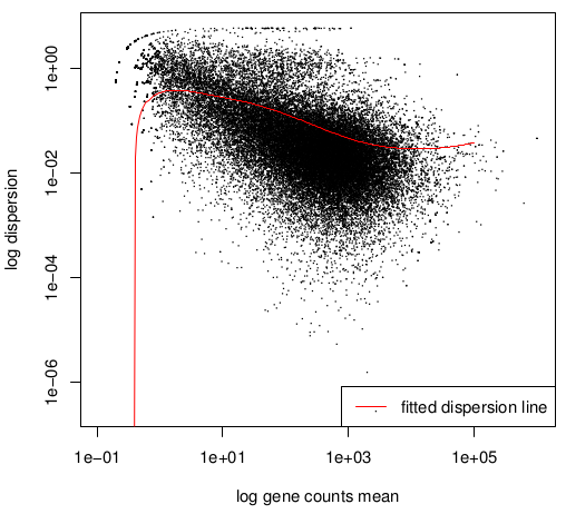
Normally the dispersion decrease when count value increase, that is why the black "cloud" (draft estimation values) and the red curve (fitted value) must be decreasing.

MA-plot

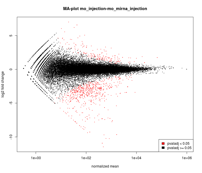
The main DESeq assumption is that most of genes are NOT differentially expressed. It is possible to verify this assumption on this graph : most of points must be black and near to 0 on the vertical axis.

Raw p-value distribution barplot

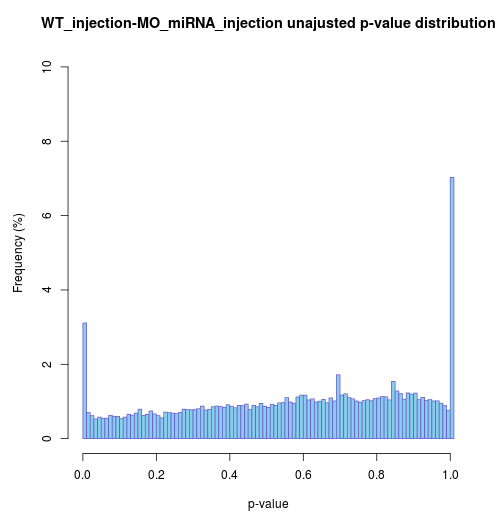
If the differential analysis performed well, raw p-value except ends would be almost uniform.